This is a toy analysis to see how grouping might affect generalization capabilities of a population. Here generalization for a population corresponds to being able to survive changes in the cost function. In such situations, a more diverse population is beneficial because of the range it covers in the fitness landscape. In a system without any control on the actual environment, grouping (sharing fitness), provides a control on the apparent environment so that a trade off option between preserving diversity and evolution speed becomes viable.
So I recently was reading a bit about the question of how a fundamental unit of selection can results in grouping at higher levels. As an example, eusociality in insects involves extensive hierarchy creation and role division with intra-group altruistic behavior as an identifying trait. A simple explanation is provided just by considering the gene level of selection and applying Hamilton's rule hamilton1964genetical (though its not exactly right) which provides a connection between how much an individual should be willing to sacrifice in order to cause net benefit to his/her genes.
There are other game theoretic models which offer interesting explanations of different collective behaviors. In chastain2014algorithms, the authors present a multiplicative weight update algorithm for modeling sexual reproduction which results in diversity preservation in the population. A stochastic game based model is provided in traulsen2006evolution that explains cooperation. In general, evolutionary game theory provides explanations for various group behaviors in a population and helps explain how a certain strategy comes to be stable by modeling evolution as a game among the individuals.
The idea in this page is to understand how grouping, in general, affects the process in an evolutionary algorithm setting without any (explicitly) competitive game. In the process, we define and work with a new setting which is similar to online setting but more suitable for evolution in the biological sense. Finally, we show how these groupings help in regularizing the algorithm along with a new way to look at crossover.
1. Evolutionary Algorithms (EAs)
Using a very generic outline, we can define an EA as doing the following:
- Figure out a way to represent the solutions of the optimization problem using a simple scheme like concatenating bitstrings for all the tunable parameters.
- Start with a population of randomly initialized solutions.
- Evolve and filter out the solutions using an operation set which models, in some ways, the ideas behind natural evolution.
- Continue evolution until the solution (best or with required fitnes) is found in the current population.
Employing the vocabulary from biology, the solution encoding is referred to as genotype and its preimage is called phenotype. The evolution process works on the genotype level.
Almost all variants of these methods differ only in step 3 which defines how the population moves from one time step to other. As an example, the operation set in Genetic algorithm (GA), which is based on ideas behind sexual reproduction, is a mixture of mutation (random changes in solution encoding), crossover (some form of mixing between two solutions) and fitness based filtering (e.g., pick \(n\) best individuals among the population, their mutants and the crossed over descendants).
Another example to give a sense of variations in these techniques is an algorithm called \((1 + 1) ES\) (Evolution Strategies) which is similar to hill climbing. In this, the population size is 1 and it evolves using only mutation. If the mutant it generated is better, then the current (only) solution in the population is replaced by the mutant.
2. Generalization
Generalization in a regular EA (solving an optimization problem) refers to ability of the algorithm to work well beyond the data set its trained on. Although EAs can be seen as optimization techniques based on evolution, there are a few differences between these and real evolution:
- The cost function in real evolution is not static.
- Training in real evolution doesn't provide that much control over the hyper parameters in optimization (like time of evolution).
It can be said that the solutions in evolution are for a different problem. This also changes the meaning of generalization a bit in evolution, which we will come back to later.
3. Shifting landscapes
Instead of working in a batch or online setting looking for a single solution, we can think of evolution as trying to solve an episodic survival problem. The setting is similar to online setting, but differs in the following ways:
- There is no single cost function to optimize. The time dimension encodes episodes which are a zone of defined cost function (defining a fitness landscape).
- A good solution to an episode's cost function might not be good for the next episode. The population thus only wants to do well in the current episode's cost function.
To elaborate, consider a learning problem for a computer game having different levels \(L_i\) with different set of possible training samples \(S_{L_i}\). For building an agent which does good on all the levels, the usual learning settings do fine. But if we only care about traversing through the levels once and we are guaranteed that the levels don't repeat, a better solution will be to only consider the loss on current level while optimizing the parameters of the learning agent.
In some ways, this tries to approximate the ideas behind real evolution where a population is faced with changing conditions. In that case, species fit for (say) \(CO_2\) based atmosphere will not survive if a reversal event like the Oxygen holocaust takes place, increasing the \(O_2\) concentration at the cost of \(CO_2\).
This also generalizes the train-test split method in which a learner must learn on training data but perform well on testing data. Other than effectively being a chain of such splits, a difference here is that the two splits are not guaranteed to be from the same distribution and so are more flexible in terms of how far the episodes can jump.
In this setting, generalization means how well a population does if faced with change in episode. If we have an ideal, all-knowing, algorithm for stepping the population, the population will move to the peak of each episode's cost function in one time step and stay there, reaping the benefits, until the next episode switch. But any practical survival (non oracle-ish) algorithm will have constraints on how far it can move the population in one time step just because it doesn't know the truth. This leads to a potential regularization strategy which provides a trade off between overfitting an episode greedily and trying to be open enough for the next ones.
The next section presents the population model, the fitness landscape and constraints that we are going to work with.
3.1. Population Dynamics
We adopt the selfish gene worldview williams1997adaptation for our problem. This means that in our world, genes are the fundamental units of selection and, in absence of any interaction, they are judged and filtered using their own fitness values.
A population of genes at time \(t\) is a multiset of size \(n(t)\) containing all the genes alive at the time. Each gene \(g_i \in p(t)\) has a chance of surviving at time \(t\) so that it stays alive at time \(t+1\) too. This survival probability is given by \(SP(g_i, Loc(g_i), Agg(g_i))\). We will use a shorthand \(s_{g_i}\) (or just \(s\), if the context is clear) meaning the survival probability of \(g_i\).
Notice that other than the index \(i\) identifying it, the gene also has a proper location in the fitness landscape which is defined by the function \(Loc(g_i)\). The function \(Agg(g_i)\) captures the effect of other genes in the population. In the case with no intra-population interaction, \(Agg(g_i) = 0\). An important point to note here is that \(SP\) is defined by \(Loc\) (ignoring \(Agg\) for a moment) but it can be different if other effects factor in (we will see an example later). Thus there really are two fitness landscapes,
- Actual landscape: Defined by \(Loc\) function.
- Apparent landscape: Defined by \(SP\) function.
An important consequence of this is that to survive, a gene does not need to do well in actual landscape if the apparent landscape is conducive. The term landscape will refer to the actual landscape from here on unless explicitly stated.
Other than the survival specification, we also have a max capacity (\(K\)) on how many genes can be in a population. If the population size, \(n\) exceeds this capacity then the genes with lower fitness are culled to make the population size equal \(K\).
To move the population, we now add a mutation function \(M(g_i, m)\). This function takes in a gene and returns a new, mutated, gene based on the original \(g_i\) with probability \(m\). This new individual is now a part of the population. To see how this helps in motion, consider a population \(p(t)\) of size \(n(t) = 1\) with a constant survival probability \(s = 0.5\). At the time step \(t\), if survived, the (only) individual in the population either does nothing or begets another individual at a nearby location. If the nearby location has higher value of \(s\) (say 1), then the population has effectively shifted towards that location.
This can be formalized in a simple way using a one dimensional landscape explained later.
4. δ-landscape
We assume a mutation model similar to wright1932roles which effectively considers mutations of a gene as a set of its neighbours which are reachable in a single step using the outgoing connections from the current gene. For our purpose, this means that the continuous fitness landscape of dimension \(d\) is broken down in a discrete mesh of certain step size. A mutation now is a movement operator which moves a single step (no diagonals) on this grid.
We can define a one dimensional fitness landscape by locally approximating it as linear surface with a slope \(\delta\). This means a gene at position \(p\) with survival probability \(s\) will go to either \(p + 1\) (\(s \rightarrow s + \delta\)) or \(p - 1\) (\(s \rightarrow s - \delta\)).
4.1. \(\delta = 0\)
Consider a case with \(\delta = 0\), i.e. the uniform fitness landscape. In this case, mutation doesn't matter since all locations in the landscape are equivalent with respect to the value of \(s\). Starting with a population of size \(n(t)\) at time \(t = 0\), population (in expectation; we work with expectations from here on) at time \(t = 1\) can be given as:
\[ n(1) = n(0) 2 s \]
More generally, the population at any time \(T\) is given as:
\[ n(T) = n(0) (2 s)^T \]
The factor of 2 comes in because, if survived, each individual splits in two (one original and another mutation). As an aside, the relation above sets the population to be exponentially increasing if \(s > 0.5\). This is not an issue since there is already a culling mechanism in place which takes the top \(K\) individuals at each evolution step.
4.2. \(\delta \ne 0\)
Let's assume \(\delta > 0\). In this case, starting with a population of size \(n\) concentrated at a position \(p\) with survival probability \(s\), a time step will spread the population at three locations using the following steps:
- Survival: Out of \(n\), \(ns\) will survive.
- These \(ns\) will clone themselves to become \(2ns\).
- From the \(ns\) clones, \(m\) will be mutated. This leaves \(ns(2 - m)\) individuals at the original position \(p\).
- From the \(snm\) mutants, \(1/2\) will go uphill in the fitness landscape and other half will move down.
- The three positions \(p - 1\), \(p\) and \(p + 1\) now have \(snm/2\), \(ns(2 - m)\) and \(snm/2\) individuals respectively.
Although this split is symmetrical, the next split won't be because the value of \(s\) at the same three positions is not symmetrical. Those \(s\) values in this case are \(s - \delta\), \(s\) and \(s + \delta\) respectively. This causes uphill population to flourish more than the downhill.
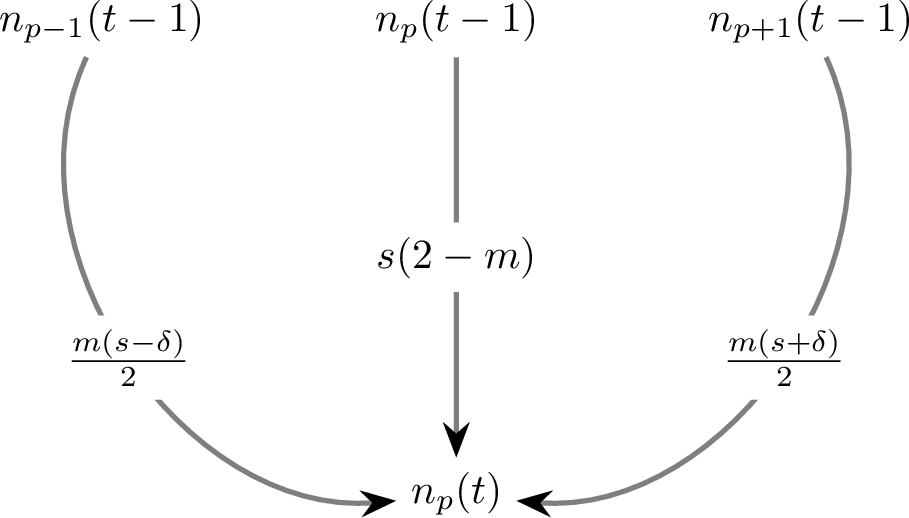
In the general case, the number of individuals at position \(p\) with survival value \(s\) and time \(t\) is dependent on individual counts at positions \(p - 1\), \(p\) and \(p + 1\) at time \(t - 1\) and can be given as:
\begin{align*} n_p(t) &= n_{p - 1}(t - 1) \frac{m (s - \delta)}{2} \\ &+ n_p(t - 1) s (2 - m)\\ &+ n_{p + 1}(t - 1) \frac{m (s + \delta)}{2} \end{align*}Since we are constrained to choose just the top \(K\) items from the population at any time, we only need to notice the rightmost (assuming +ve δ) part of this count distribution in the set of all (\(2t + 1\)) possible positions at time \(t\). Using the above recursive equation, an simple case is of the rightmost fringe at each time step which just depends on the one of the terms. This is given by \(n_{right}\):
\begin{align*} n_{right}(t) &= n_{right}(t - 1) \frac{m (s_{n_{right}(t-1)} + \delta)}{2} \\ \end{align*}Starting with \(n\) individuals at time 0 at the same position with survival value of \(s\), \(n_{right}\) can be reduced to:
\begin{align*} n_{right}(t) &= n (\frac{m}{2})^t \Pi_{i = 0}^t (s + i \delta) \end{align*}In general, a higher value of δ (meaning steeper landscape) will increase the number of individuals in the same (in the right side of the original \(s\)) spots considering all factors to be the same.
5. Improving generalization
Coming back to the question of generalization, there are two things to point out here:
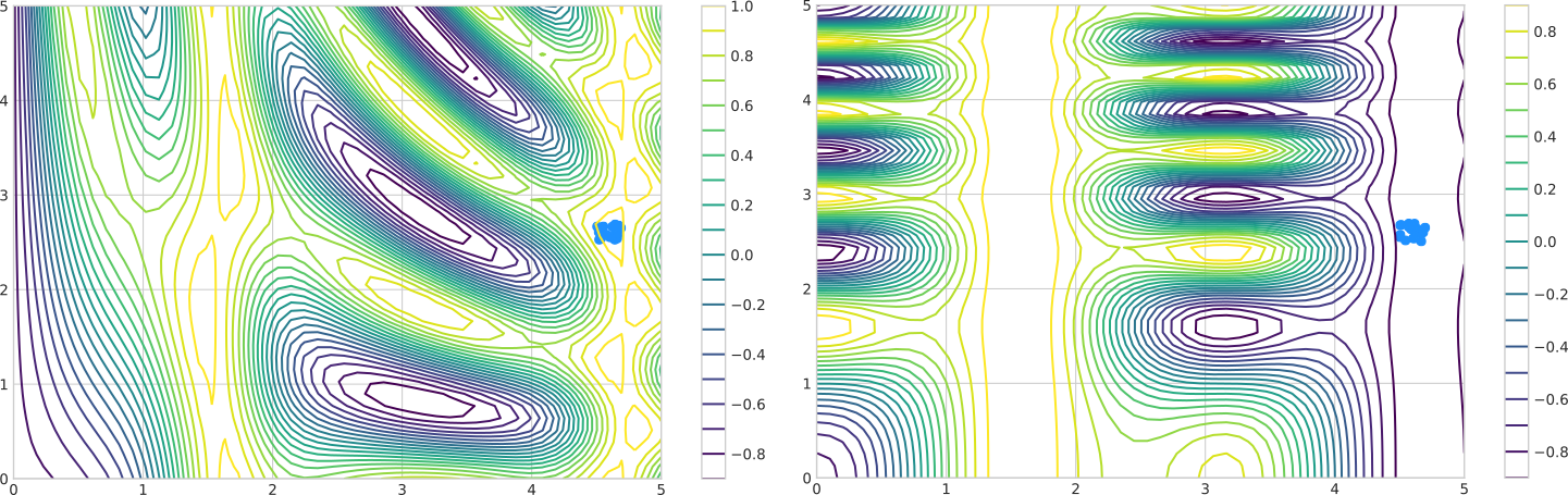
- If there are two scenarios with the same number of genes but with different distribution of counts, a more diverse distribution has higher chance of surviving any change in landscape.
- Because of higher population count in the high δ case, we get a smaller span of active positions (positions with non-zero population) after culling for top \(K\) items.
In effect, if the situation is good for survival, and we are hitting the culling capacity (so that the two scenarios have same population counts), a low value of δ will make the population more spread out than a higher one. This, in turn, makes the population in low δ world preserve more diversity and survive better in case of a switch of landscape resulting in a more generalized solution.
Adding to these the constraints that we don't actually have control over either the time of evolution \(t\), the value of δ or mutation rate \(m\) if we are in the population (this assumption doesn't really work if we go on a much longer scale and make mutation itself evolvable), what might be a good strategy to improve generalization?
5.1. Changing slope by grouping
Although the value of δ for the actual landscape can't be changed, the value of δ for the apparent landscape can be changed by appropriate interactions among the individuals.
This brings us to the \(Agg\) function which changes the value of \(SP\) using the effects from inter individual interactions. Consider a sharing strategy where the function groups \(k\) individuals, takes the mean of their actual fitness values and assigns this mean as the apparent fitness of all the individuals. In the extreme case of \(k = n\), this makes the apparent value of δ to be 0. On the other hand, with \(k = 1\), this reduces to situation with no interaction and apparent δ equals actual δ. By varying \(k\), apparent slope can be controlled. A higher \(k\) value provides more flatness and thus adds inertia.
5.2. Crossover
Crossover acts as a technique to swap chunks of genes among organisms. Considering 'organisms' as groups of genes we create in this case, crossover can be seen as a trick to reduce the δ value as its effect is to shuffle genes around groups. Whatever way maybe used to form initial groups, a random shuffling operator like crossover is going to increase the flatness in expectation. Thus it can be seen as a way to flatten the landscape without increasing the \(k\) value.
Computational modeling of evolution is a really nice way to play around with and understand some of the major ideas. Although this experiment says nothing conclusively (there are sufficiently high quantities of assumptions and cherry-picking), it showed me a lot of directions to pursue for getting to the right way of modeling the processes.
An important point from my perspective is to see connnections between life processes and computation (which, when applied to biological world, ends up sharing a lot of pieces with machine learning). As a next step, I would like to spend time understanding the equivalences (if there are) between biological terms like robustness and learning stability. The hostility of real environment throws challenges like population bottleneck which are sufficiently different than the simple learning settings we work with regularly and thats pretty interesting.